by R. Grothmann
The following problem seems to go back to Phillip Apian (1531-1589), a German geometer:
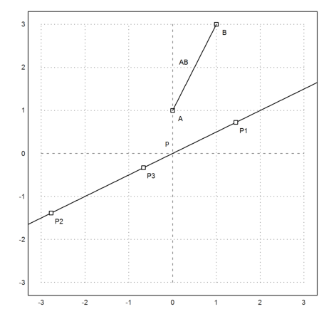
"Search the point on a line such that a given line segment appears at a maximal angle.
Philipp Apian on German Wikipedia
In poetic form, he asked at what distance a man sees most of his beloved standing on a balcony. That is a special case where the line is orthogonal to the segment.
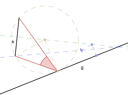
The sketch shows the solution in the given situation, and it also shows the idea of the general solution. The circle is constructed such that it goes through the endpoints of the segment, and touches the line. The construction has been done by C.a.R.
The angle of the segment is the same for all points on the circle, larger for points inside the circle, and less for points outside the circle. Thus it is clear why the circle touching the line provides the optimal angle.
Can you see the construction of this circle, indicated in the sketch?
There is a very easy geometric solution.
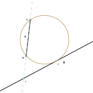
Based on the secant-tangent-theorem we have
![]()
Thus AD can be constructed.
E.g. in the special situation
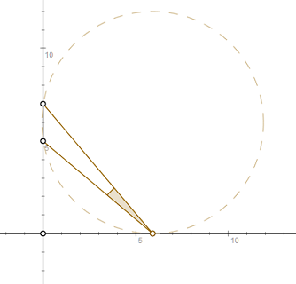
We easily get the point
![]()
This can also be derived analytically by maximizing the angle.
>f &= atan(7/x)-atan(5/x)
                               7         5
                          atan(-) - atan(-)
                               x         x
>&solve(diff(f,x))
[x = - sqrt(35), x = sqrt(35)]
Let us try our library "geometry.e".
>load geometry;
We solve a special case analytically, neglecting the geometric solution we already have.
The file geometry.e contains commands for analytic geometry, both numerically, and symbolically.
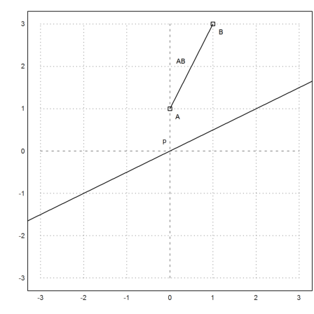
First we set the points in Euler, and in Maxima.
>A &:= [0,1]; B &:= [1,3];
Now we set the plot range.
>setPlotRange(-3,3,-3,3);
The plot commands in geometry always add elements to the plot.
We add the two points, and the segment through these points.
>plotPoint(A,"A"); plotPoint(B,"B"); plotSegment(A,B);
Then we define a line in Euler and Maxima, and add it to the plot.
>l&:=lineWithDirection([0,0],[2,1]); plotLine(l):
Maxima can extract the equation of the line from the line vector.
>le &= getLineEquation(l,x,y)
2 y - x = 0
In the next step, we compute the quadrances of the segment, and the distance from a point [x,y] to A and B. Quadrances are distances squared. These terms are explained in the example about "Rational Geometry" (search the internet for Normal Wildberger).
>s&=quad(A,B), a&=quad([x,y],A), b&=quad([x,y],B)
                                  5


                                   2    2
                            (1 - y)  + x


                                2          2
                         (3 - y)  + (1 - x)
The spread of the angle at [x,y] satisfies the "crosslaw", a translation of the cosine law into rational geometry. The spread of an angle t is defined as sin(t)^2. Maxima can be used to setup the equation of the crosslaw for our situation, and it can solve the equation fot this spread.
We create a function w(x,y), which returns the spread for each point [x,y].
>&crosslaw(s,a,b,w), &solve(%,w); function w(x,y) &= factor(rhs(%[1]))
                2          2    2          2     2
        ((3 - y)  + (1 - y)  + x  + (1 - x)  - 5)  =
                                         2    2          2          2
                       4 (1 - w) ((1 - y)  + x ) ((3 - y)  + (1 - x) )


                                         2
                            (y - 2 x - 1)
            ----------------------------------------------
              2          2               2          2
            (y  - 6 y + x  - 2 x + 10) (y  - 2 y + x  + 1)
This is a nasty function.
![]()
It is in fact the square of the sine of the angle at [x,y] at which the segment appears.
We now wish to maximize w(x,y) under the condition that [x,y] is on our line. We use the Lagrange formula for this, but we could just as well substitute y=x/2. Surprisingly, Maxima finds all solutions.
>sol &= solvelagrange(w(x,y),lhs(le),[x,y])
                                              3/2
                          sqrt(6) I + 3      2    sqrt(3) I + 6
        [[lambda = 0, y = -------------, x = ------------------],
                                5                    5
                                         3/2
                 3 - sqrt(6) I      6 - 2    sqrt(3) I
[lambda = 0, y = -------------, x = ------------------],
                       5                    5
                 9/2  5/2
           7209 2    5    - 9298800        sqrt(10) - 1
[lambda = ---------------------------, y = ------------,
                15/2  9/2                       3
          2611 2     5    - 661422500
     3/2                                9/2  5/2
    2    sqrt(5) - 2              7209 2    5    + 9298800
x = ----------------], [lambda = ---------------------------,
           3                           15/2  9/2
                                 2611 2     5    + 661422500
                           3/2
    - sqrt(10) - 1      - 2    sqrt(5) - 2
y = --------------, x = ------------------],
          3                     3
                   1        2
[lambda = 0, y = - -, x = - -]]
                   3        3
Now we extract the real solutions to Euler. The result are three points.
>P1 := &at([x,y],sol[3])(), plotPoint(P1,"P1"); ...
 P2:="::at([x,y],sol[4])"(), plotPoint(P2,"P2"); ...
 P3:="::at([x,y],sol[5])"(), plotPoint(P3,"P3"); ...
 insimg;
[1.44152,  0.720759]
[-2.77485,  -1.38743]
[-0.666667,  -0.333333]
In fact, these points are local extrema. Two of them are solutions of touching circles, and one is the intersection of the line through AB with the given line.
>color(4); ...
 plotCircle(circleThrough(A,B,P1)); ...
 plotCircle(circleThrough(A,B,P2)); ...
 plotLine(lineThrough(A,B)); ...
 color(1); ...
 insimg;
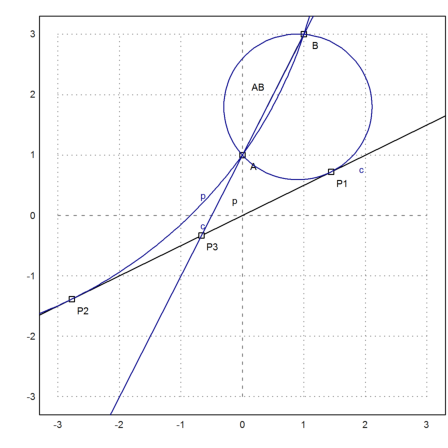
Note that P3 is an extremal point, since our spreads are always positive, and the angle is 0 there.
Let us plot the function w(x,y), when [x,y] walks along the line. First we make a function w1(x).
>&solve(le,y); function w1(x) &= factor(w(x,at(y,%)))
                                       2
                            4 (3 x + 2)
                  ---------------------------------
                      2                2
                  5 (x  - 4 x + 8) (5 x  - 4 x + 4)
Then we plot it.
>plot2d("w1(x)",-5,5); ...
 t=[P1[1],P2[1],P3[1]]; plot2d(t,"w1(t)"(),points=1,add=1):
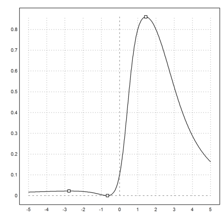
We can see the three local extrema. Of course, P1 is the point, we are looking for.